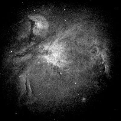
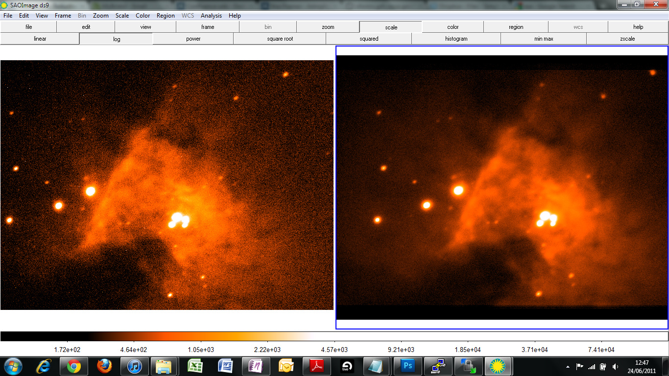
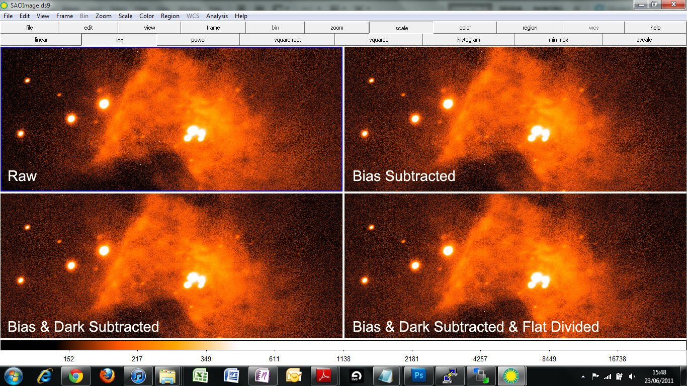
Figure 1: A raw image of M42 (the Orion Nebula) and the image after each subsequent data reduction process. In this example there is negligible visual impact, however the resulting FITS file flux values will be a far truer representation. (click for expanded view)

The data reduction process is important for photometry as the contributions from dark current, bias and flat field alter the number of counts in a frame and so correcting for these may not present a significant visual difference (as is the case with Fig. 1 on the right), however a calculation of flux will be more accurate.

Step-by-step:

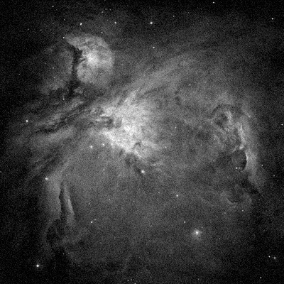
The general process for data reduction is outlined below with the aid of exaggerated mock results for illustrative purposes (image of M42 taken by the Hubble Space Telescope. Credit: NASA/ESA).

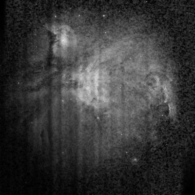	The raw file as retrieved from the CCD. It includes all contributions from dark current, bias and flat field. Important information that must be retained when working with the image are the exposure length and cooling temperature of the CCD when the image was taken. This data is usually stored in the FITS file header.
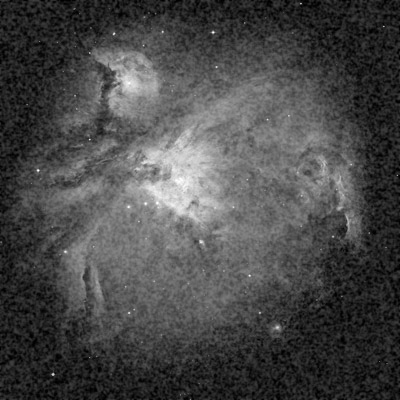	The first step to data reduction is to subtract a master bias frame for the same CCD temperature as the image. The bias contribution is independent of exposure length and so must be subtracted before performing any scaling. The mock bias that has been subtracted in this example is below: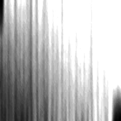
	Next, a model of the dark current's contribution must be subtracted (master dark subtraction). This master dark frame is a long dark exposure with the bias subtracted. It is then divided so that its effective exposure length matches that of the data image and subtracted from it. The mock dark frame that has been subtracted in this example is below:
	Finally, the image must be divided by the master flat frame. This removes any artefacts present due to uneven illumination of the CCD (generally vignetting due to the telescope). The mock bias that the image has been divided by in this example is below: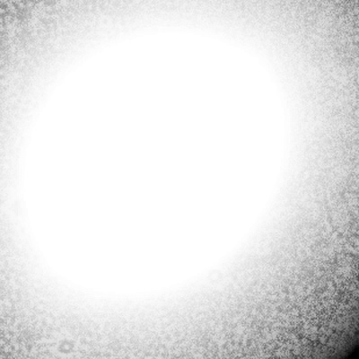

Stacking:

In some situations (particularly when observing extended objects) the object you wish to image is much fainter than another bright object in the field of view or the object just has a very large range of intensities. This raises issues because the brighter part of the image may saturate quickly leaving a very low S/N ratio in the fainter areas. It is when this occurs that stacking becomes useful.

By taking multiple exposures of maximum length before saturation occurs, aligning each one (this is called registering) and then adding the images together, one can acquire a much longer exposure image thereby enhancing detail in fainter regions.

In pseudo-code, the process would look as follows:

 FIND x-y coords of brightest star for ALL FILES
 Width diff = max x-coord - min x-coord
 Height diff = max y-coord - min y-coord
 Make 3d array [image width + width diff, image height + height diff, number of files to stack]
 FOR n=1 to number of files BEGIN
    3D array[*,*,file number] = file 'n' offset by (max x-y coords - star x-y coords for file 'n')
 ENDFOR
 SUM 3d array over 3rd dimension

The result should be a merged 2D array larger than each image with effective exposure length equal to the sum of all the exposure lengths. Noise compared to signal in the dimmer parts should be much less.
An example of this performed successfully with the Coldrick Observatory as part of the 2010-11 project is shown below in Fig. 2:

Figure 2: An example of the effect of stacking images. One raw image of M42 is shown on the left, 7x similar 5 second images were stacked to produce the image on the right. Note that some faint stars within the gas are apparent only on the stacked image; also note the large reduction in noise, producing a much smoother image.

datareduction.jpg (image/jpeg)
Bias.jpg (image/jpeg)
DC.jpg (image/jpeg)
flat.jpg (image/jpeg)
BiasSub.jpg (image/jpeg)
DCSub.jpg (image/jpeg)
FlatSub.jpg (image/jpeg)
Raw.jpg (image/jpeg)
stacking.jpg (image/jpeg)